Skewness calculation with Python

Skewness is a statistical measure that describes the skewness of the distribution of a data set. Indicates whether the tail of the distribution is shifted to the left or to the right compared to its central part. Positive skewness indicates a longer tail on the right, while negative skewness indicates a longer tail on the left.

[wpda_org_chart tree_id=16 theme_id=50]

The Skewness

Skewness is a crucial measurement that helps us understand how much our data is skewed left or right relative to its mean. When skewness is positive, it suggests that there may be exceptionally high values affecting the right tail of the distribution. Conversely, negative skewness indicates a longer tail on the left, suggesting possible lower outlier values. This information is fundamental in data analysis as it provides insights into the shape of the distribution, also guiding the choice of appropriate statistical techniques and facilitating the prediction of the future behavior of the data. Additionally, skewness is useful in detecting outliers, comparing distributions, and describing the concentration of data around the mean. In summary, it is a valuable tool for interpreting data structure and driving informed statistical analyses.

Skewness can be measured using several formulas, but one of the most common is the third-order momentum formula. If we denote the skewness as (g_1), the formula is:

Where:

• is the number of observations in the data.
• is each observation.
• è la media dei dati.

This formula compares the third-order moment (skewness) to the square of the second-order moment (variance). The skewness will be positive if the distribution is skewed to the right, negative if it is skewed to the left, and zero if it is perfectly symmetric.

What is the point of knowing Skewness

Knowing the skewness of a distribution is useful in statistics for understanding the shape and skewness of data. Here are some reasons why this is important:

1. Description of the distribution: Skewness provides information about the shape of the data distribution. Non-zero skewness indicates that the distribution is not symmetric.
2. Behavior prediction: It can help predict how data will behave. For example, positive skewness suggests the presence of longer tails on the right, indicating the possibility of extremely high values.
3. Selection of statistical techniques: Knowledge of skewness can influence the choice of appropriate statistical techniques. Some statistical methods assume a symmetric distribution, so skewness can affect the interpretation of results.
4. Anomaly detection: In some cases, significant skewness can indicate the presence of anomalies or data outliers that could affect the analysis.

In general, skewness is a useful tool for gaining a deeper understanding of the structure and central tendency of a data set.

If you want to delve deeper into the topic and discover more about the world of Data Science with Python, I recommend you read my book:

Python Data Analytics 3rd Ed

Fabio Nelli

An example of Skewness calculation

In Python, you can use the scipy library to calculate the skewness of a data set. Here is an example of how to do it:

import numpy as np
from scipy.stats import skew

# Create a sample dataset
data = np.array([1, 2, 2, 3, 3, 3, 4, 4, 4, 4, 5, 5, 5, 5, 5])

# Calculate the skewness
skewness = skew(data)

# Print the result
print("Skewness:", skewness)

In this example, I used a simple data set, but you can replace the data array with your own data set. The skew function will return the skewness calculated for that data. Running the code you will get the following result:

Skewness: -0.5879747322073333

Some examples of application of Skewness

Skewness in the study of a distribution

Here’s an example of how you can use Python to calculate skewness and describe the shape of a distribution:

import numpy as np
from scipy.stats import skew
import matplotlib.pyplot as plt
import seaborn as sns

# Create a data set with positive skewness
data_positive = np.random.exponential(scale=2, size=1000)

# Create a data set with negative skewness
data_negative = np.random.beta(a=2, b=5, size=1000)

# Calculate the skewness for both data sets
skewness_positive = skew(data_positive)
skewness_negative = skew(data_negative)

# View distributions
plt.figure(figsize=(12, 4))

plt.subplot(1, 2, 1)
sns.histplot(data_positive, kde=True, color='blue')
plt.title(f'Skewness positive: {skewness_positive:.2f}')

plt.subplot(1, 2, 2)
sns.histplot(data_negative, kde=True, color='orange')
plt.title(f'Skewness negative: {skewness_negative:.2f}')

plt.show()

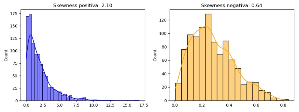
In this example, I’m creating two data sets, one with positive skewness and one with negative skewness. I’m using an exponential distribution for the former and a beta distribution for the latter. Next, I calculate the skewness for each data set and visualize the distributions using the seaborn module. The skewness is then printed in the title of each graph.

You can run this code in your Python environment to visually see how the skewness reflects the skewness of the distributions. Positive skewness is associated with a longer tail on the right, while negative skewness is associated with a longer tail on the left.

Comparison between different distributions

Here is an example of how you can use Python to calculate skewness and compare skewness between different distributions:

import numpy as np
from scipy.stats import skew
import matplotlib.pyplot as plt
import seaborn as sns

# Create two data sets with different skewness
data_set1 = np.random.normal(loc=0, scale=1, size=1000)
data_set2 = np.random.exponential(scale=2, size=1000)

# Calculate the skewness for both data sets
skewness_set1 = skew(data_set1)
skewness_set2 = skew(data_set2)

# View distributions
plt.figure(figsize=(12, 4))

plt.subplot(1, 2, 1)
sns.histplot(data_set1, kde=True, color='blue')
plt.title(f'Skewness: {skewness_set1:.2f}')

plt.subplot(1, 2, 2)
sns.histplot(data_set2, kde=True, color='orange')
plt.title(f'Skewness: {skewness_set2:.2f}')

plt.show()

# Print the skewness for comparison
print(f"Skewness of the first data set: {skewness_set1:.2f}")
print(f"Skewness of the second data set: {skewness_set2:.2f}")

In this example, I am generating two data sets with different distributions: one normal and one exponential. Next, I calculate the skewness for each data set and visualize the distributions using the seaborn module. Finally, I print the skewness to numerically compare the skewnesses of the distributions.

You can run this code in your Python environment to see how the skewness reflects the differences in the shape of the distributions between the two datasets.

Recommended Book:

If you are interested to this topic, I suggest to read this:

Practical Statistics for Data Scientists

Skewness in detecting data anomalies (Outliers)

Skewness itself is not generally used as a specific tool for detecting anomalies in data. However, skewness can be a part of a larger process of identifying outliers or anomalies. Let’s see an example of how you could use skewness along with other methods to detect anomalies using Python:

import numpy as np
from scipy.stats import skew
from sklearn.ensemble import IsolationForest
import matplotlib.pyplot as plt

# Create a data set with an outlier
data = np.concatenate([np.random.normal(0, 1, 1000), [10]])

# Calculate the skewness
skewness = skew(data)

# Use Isolation Forest to detect outliers
model_isolation_forest = IsolationForest(contamination=0.01)  # Specify the percentage of contamination
data = data.reshape(-1, 1)  # Isolation Forest requires a 2D array
model_isolation_forest.fit(dati)

# Predict outliers
predictions = model_isolation_forest.predict(data)

# View the results
plt.scatter(range(len(dati)), dati, c=predictions, cmap='viridis')
plt.xlabel('Data index')
plt.ylabel('Data value')
plt.title('Anomaly detection with Isolation Forest')
plt.show()

# Print skewness and outliers
print("Skewness:", skewness)
print("Outliers:", np.where(predictiond == -1)[0])

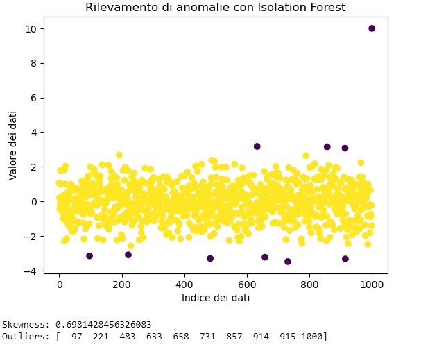
In this example, we are generating a dataset with a normal distribution and adding an outlier. Next, we calculate the skewness and use Isolation Forest to detect outliers. Finally, we visualize the data with the identified outliers.

Skewness is used here more as a descriptive measure, while Isolation Forest is used to detect actual outliers.