OpenCV & Python – The Otsu’s Binarization for thresholding

Introduction

In this article you will see how to apply another important technique with the OpenCV library – the Otsu’s binarization. This technique is very important in the analysis of images, especially in cases in which you want to apply a threshold in the thresholding techniques in an efficient manner.

The bimodal images

To apply the most of this technique, the images should be bimodal. But what is an image bimodal?

Any image is a set of dots that are defined as pixels. Each of these pixels can be represented by a triplet of RGB values in the case of a color image, and a single value if the image is in the gray scale. These values assume all values between 0 and 255. If you take all of the pixels of an image and count how many of these have value 0, how many 1, how many 2, and so on… up to 255, you get a histogram .

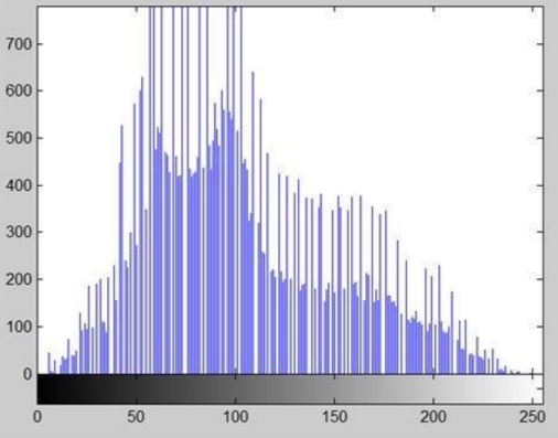
As you can see from the figure a histogram is nothing more than a way to represent the distribution of the degree of color present in an image. From the figure, for example, you can view the presence of a maximum in the middle. So in this case the image is monomodal.

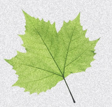
Instead image bimodal, once represented in the form of histogram, will present two separate maximum between them (modes). For example, this color image that I have made by adding a bit of background noise is a bimodal example.

Now you’ll see how to perform analysis using OpenCV to get the histogram of the image and see if the image is bimodal. Write the following program and save it as otsu01.py.

import cv2
import numpy as np
from matplotlib import pyplot as plt

img = cv2.imread('noisy_leaf.jpg',0)
plt.subplot(2,1,1), plt.imshow(img,cmap = 'gray')
plt.title('Original Noisy Image'), plt.xticks([]), plt.yticks([])
plt.subplot(2,1,2), plt.hist(img.ravel(), 256)
plt.title('Histogram'), plt.xticks([]), plt.yticks([])

plt.show()

By executing the program, the first image will be loaded in grayscale and then the histogram of the image will be generated. Displaying it immediately after the image via matplotlib you can see that the image chosen is perfectly bimodal.

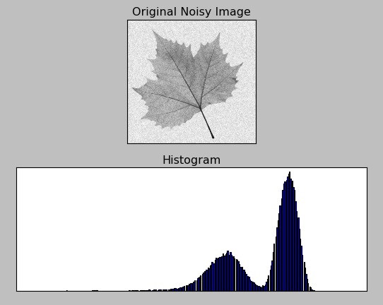
As you can see the image presents two distinct mode among them, dividing into two distinct parts the distribution of pixels in the image.

The Otsu’s binarization

Now that you’ve seen when an image is bimodal and you are in possession of the tools to recognize it as such, you can see in detail the Otsu’s binarization.

Returning to the previous figure, the bimodal image, presents the histogram into two distinct distributions, almost separable between them. In fact between the two mode there is a minimum point, where you might consider the possibility of separating the histogram into two parts. Well the Otsu’s binarization helps you to automatically get that value.

Moreover, once this technique gained there will be no need to visualize and study the histogram in order to find the point, but everything will be done automatically.

Thresholding

One of the most used techniques for the analysis of the images is that of the thresholding, ie the application of a threshold along a particular scale of values, to filter in some way an image.

One of these techniques is for example the one that converts any image in grayscale (or color) in a totally black and white image. Often this is very useful for recognizing the regular shapes, contours within an image, or even to delimit and divide zones inside, to then be used in a different way in the subsequent processing.

So applied to a histogram, you will choose a value in which all the underlying values will be converted to 0 (white) and all those overlying to 255 (black), by converting an image to grayscale into black and white.

In OpenCV to perform the thresholding you can use the cv2.threshold() function

Take the case of the image of the previous leaf. Make the case that you need to recognize the shape of the leaf, but you can not use a histogram. As a first approach you’ll try to apply a threshold (a threshold) at random, and then after several attempts able to find an optimal value.

The first value definitely worth trying is 127, which in the scale of 0-255 is perfectly in the middle. Then you apply this value to the cv2.threshold() function. Thus, write the following program and save it as otsu02.py.

import cv2
import numpy as np
from matplotlib import pyplot as plt

img = cv2.imread('noisy_leaf.jpg',0)

#ret1, th1 = cv2.threshold(img, 127, 255, cv2.THRESH_BINARY)

ret, imgf = cv2.threshold(img, 0, 255, cv2.THRESH_BINARY+cv2.THRESH_OTSU)

#blur = cv2.GaussianBlur(img, (5,5), 0)
#ret3, th3 = cv2.threshold(blur, 0, 255, cv2.THRESH_BINARY+cv2.THRESH_OTSU)

plt.subplot(3,1,1), plt.imshow(img,cmap = 'gray')
plt.title('Original Noisy Image'), plt.xticks([]), plt.yticks([])
plt.subplot(3,1,2), plt.hist(img.ravel(), 256)
plt.axvline(x=ret, color='r', linestyle='dashed', linewidth=2)
plt.title('Histogram'), plt.xticks([]), plt.yticks([])
plt.subplot(3,1,3), plt.imshow(imgf,cmap = 'gray')
plt.title('Otsu thresholding'), plt.xticks([]), plt.yticks([])
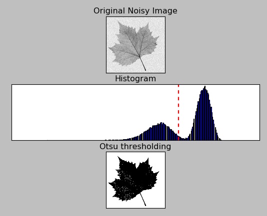
plt.show()

Execute it.

As you can see from the figure, actually the value chosen at random is completely out of the desired value, and the only picture you see are the large veins of the leaf.

At this point you choose the threshold values by trial and error, but it would take time. It would be better if you could view the histogram and choose a minimum value between the two modes. In fact, even in this case the value you’ve chosen would not be the optimal one (in fact the lowest value not always is the correct threshold), but one that takes into account the weights of the distributions. Also often the situation of the histograms is not so clear …

The Otsu’s binarization

Here comes the Otsu’s binarization. This algorithm will allow you to quickly and automatically obtain the correct threshold value to choose between two histogram mode, so as to apply the thresholding in an optimal manner.

In OpenCV, the application of the Otsu’s binarization is very simple. It will be sufficient to add as parameter within the cv2.threshold () function, called

cv2.THRESH_OTSY

Now you can write the following code, and save it as otsu03.py.

import cv2
import numpy as np
from matplotlib import pyplot as plt

img = cv2.imread('noisy_leaf.jpg',0)

ret, imgf = cv2.threshold(img, 0, 255, cv2.THRESH_BINARY+cv2.THRESH_OTSU)

plt.subplot(3,1,1), plt.imshow(img,cmap = 'gray')
plt.title('Original Noisy Image'), plt.xticks([]), plt.yticks([])
plt.subplot(3,1,2), plt.hist(img.ravel(), 256)
plt.axvline(x=ret, color='r', linestyle='dashed', linewidth=2)
plt.title('Histogram'), plt.xticks([]), plt.yticks([])
plt.subplot(3,1,3), plt.imshow(imgf,cmap = 'gray')
plt.title('Otsu thresholding'), plt.xticks([]), plt.yticks([])
plt.show()

By running the code this time you’ll get the best results. In addition it is possible to see which is the optimal threshold value found by Otsu’s binarization within the histogram. As you can see it is between the two modes, but not in the minimum point.

The algorithm: How works the Otsu’s binarization

Since you’re working with images bimodal, the Otsu’s algorithm will try to find the threshold value t that minimizes the weighted within-class variance, defined as a weighted sum of the variances of the two classes:

where

and

and

In Internet I found the following code (see here) to implement the mathematical expressions given above in the algorithm and performs all necessary calculations. However I had to put some changes since it generated some errors, such as division by zero. Write it down and save it as otsu04.py.

import cv2
import numpy as np

img = cv2.imread('noisy_leaf.jpg',0)
#blur = cv2.GaussianBlur(img,(5,5),0)

# find normalized_histogram, and its cumulative distribution functio
hist = cv2.calcHist([img],[0],None,[256],[0,256])
hist_norm = hist.ravel()/hist.max()
Q = hist_norm.cumsum()
bins = np.arange(256)
fn_min = np.inf
thresh = -1
for i in xrange(1,256):
 p1,p2 = np.hsplit(hist_norm,[i]) # probabilities
 q1,q2 = Q[i],Q[255]-Q[i] # cum sum of classes
 if q1 == 0:
    q1 = 0.00000001
 if q2 == 0:
    q2 = 0.00000001
 b1,b2 = np.hsplit(bins,[i]) # weights
 # finding means and variances
 m1,m2 = np.sum(p1*b1)/q1, np.sum(p2*b2)/q2
 v1,v2 = np.sum(((b1-m1)**2)*p1)/q1,np.sum(((b2-m2)**2)*p2)/q2
 # calculates the minimization function
 fn = v1*q1 + v2*q2
 if fn < fn_min:
    fn_min = fn
    thresh = i
# find otsu's threshold value with OpenCV function
ret, otsu = cv2.threshold(img,0,255,cv2.THRESH_BINARY+cv2.THRESH_OTSU)
print thresh,ret

But if I run the program, the results of the two threshold are not exactly alike

204 202.0

Conclusions

In this article you saw how to apply the best way of thresholding technique in the case of bi-modal images, and this is thanks to the binarization of Otsu’s binarization. In more articles to come, other techniques with respect to the thresholding will be explored using the OpenCV library on Python.[:]