


The Probability Density Function (PDF) is a mathematical function that describes the relative probability of a random variable taking on certain values. In other words, it provides a representation of the probability distribution of a continuous variable. The PDF is non-negative and the area under the curve is 1, as it represents the total probability. For example, in the normal distribution, the PDF is represented by a bell curve.
The Probability Density Function
The Probability Density Function (PDF) is a function that describes the probability distribution of a continuous random variable. The PDF is often denoted as (f(x)), where (x) represents the value of the random variable.
PDF equation:
The specific form of the equation depends on the distribution of the random variable. For example, for the standard normal distribution, the PDF is:


Where:


This PDF describes the shape of the classical Gaussian bell. The PDF is therefore a key tool for understanding and working with continuous random variables, allowing you to make predictions, calculate probabilities and analyze the shape of the probability distribution.
The derivation of the PDF depends on the specific distribution of the random variable. In some cases, it can be derived from the Cumulative Distribution Function (CDF).
Utilities of PDF
- Probability Calculation: The area under the PDF curve in an interval corresponds to the probability that the random variable falls in that interval. This is achieved by integrating the PDF over that range.
- Calculating Statistics: The PDF allows you to calculate various statistics, such as mean and variance, by integrating the appropriate expressions on the PDF.
- Predictions and Analysis: The shape of the PDF provides information about the distribution of the random variable. For example, in the normal distribution, a bell-shaped PDF indicates that central values are more likely than extreme values.
- Comparison of Distributions: Can be used to compare different distributions and understand how the probabilities change in different regions of the random variable.
In essence, PDF is a fundamental tool for understanding and working with continuous random variables, providing a detailed description of the probability distribution and enabling a wide range of statistical analyses.


Recommended Book:
If you are interested to this topic, I suggest to read this:
Some examples in Python
Here are some code examples involving the Probability Density Function (PDF) for some common distributions using the Python language with the SciPy library:
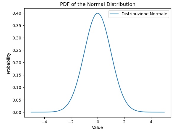
Normal Distribution
The most commonly used probability distribution is that of the normal distribution. The following code allows us to calculate it and display it in a graph.
import numpy as np
import matplotlib.pyplot as plt
from scipy.stats import norm

mu, sigma = 0, 1  # Mean and standard deviation
x = np.linspace(-5, 5, 1000)
pdf = norm.pdf(x, mu, sigma)

plt.plot(x, pdf, label='Distribuzione Normale')
plt.title('PDF of the Normal Distribution')
plt.xlabel('Value')
plt.ylabel('Probability')
plt.legend()
plt.show()
Running the code we obtain the following graph which corresponds to the PDF of the normal distribution
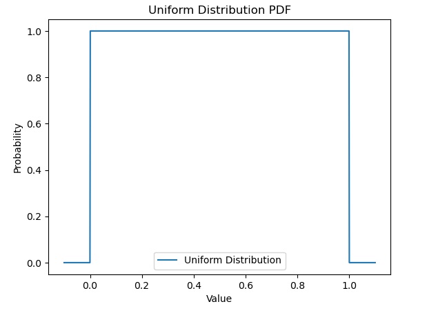
Uniform Distribution
Another well-known and used probability distribution function is that relating to the uniform distribution. The PDF for a random variable (X) with uniform distribution between (a) and (b) is defined as follows:


where 


This equation represents the constant probability density between
import numpy as np
import matplotlib.pyplot as plt
from scipy.stats import uniform

a, b = 0, 1  # Extrema of the interval
x = np.linspace(a - 0.1, b + 0.1, 1000)
pdf = uniform.pdf(x, a, b - a)

plt.plot(x, pdf, label='Uniform Distribution')
plt.title('Uniform Distribution PDF')
plt.xlabel('Value')
plt.ylabel('Probability')
plt.legend()
plt.show()
Executing you obtain the following graph.
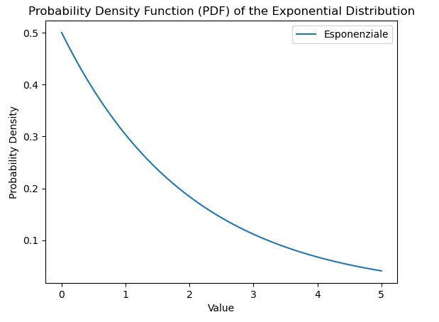
Exponential Distribution
Another widely used distribution is the exponential one. The PDF for a random variable (X) with an exponential distribution is given by:


Where 


import numpy as np
import matplotlib.pyplot as plt
from scipy.stats import expon

# Parameter of the exponential distribution
lambda_param = 0.5

x = np.linspace(0, 5, 1000)
pdf = expon.pdf(x, scale=1/lambda_param)

plt.plot(x, pdf, label='Esponenziale')
plt.title('Probability Density Function (PDF) of the Exponential Distribution')
plt.xlabel('Value')
plt.ylabel('Probability Density')
plt.legend()
plt.show()
By running the code you obtain the representation of the PDF in the following graph.
Gamma Distribution
Yet another distribution is the gamma one. Here too in this case is the code to obtain your PDF. The PDF for a random variable 


Where 


import numpy as np
import matplotlib.pyplot as plt
from scipy.stats import gamma

# Parameters of the gamma distribution
alpha = 2
beta = 1

x = np.linspace(0, 10, 1000)
pdf = gamma.pdf(x, alpha, scale=1/beta)

plt.plot(x, pdf, label='Gamma')
plt.title('Probability Density Function (PDF) of the Gamma Distribution')
plt.xlabel('Value')
plt.ylabel('Probability Density')
plt.legend()
plt.show()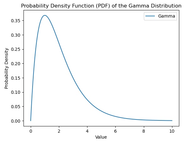


If you want to delve deeper into the topic and discover more about the world of Data Science with Python, I recommend you read my book:
Fabio Nelli
Log-Normal Distribution
To conclude, let’s also look at the Log-Normal probability distribution function. The PDF for a random variable (X) with log-normal distribution is given by:


Where 


import numpy as np
import matplotlib.pyplot as plt
from scipy.stats import lognorm

# Parameters of the log-normal distribution
mu = 0
sigma = 0.1

x = np.linspace(0, 3, 1000)
pdf = lognorm.pdf(x, sigma, scale=np.exp(mu))

plt.plot(x, pdf, label='Log-Normale')
plt.title('Probability Density Function (PDF) of the Log-Normal Distribution')
plt.xlabel('Value')
plt.ylabel('Probability Density')
plt.legend()
plt.show()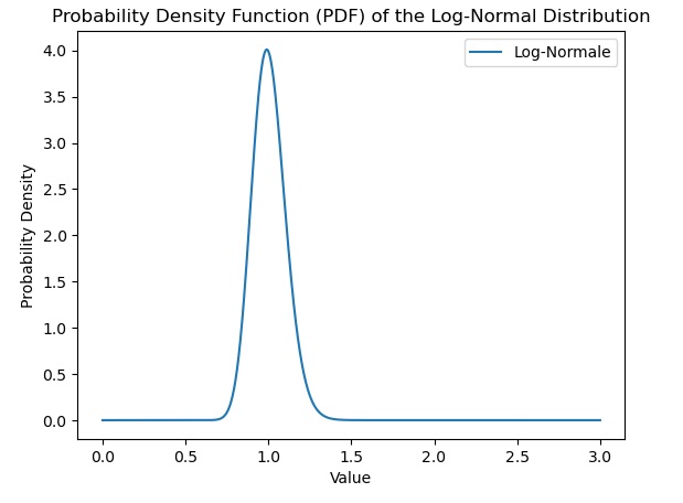
These are just a few examples of continuous distributions that can be explored using the SciPy library in Python. Each distribution has its own specific parameters that can be adapted according to the needs of the analysis.