Being able to work with data, import them, export them and other similar operations, is a very important operation to start working and performing statistics and data analysis. Here are some fundamental concepts and operations that allow you to convert external data in different formats into data frames, or in any case into types of data that can be easily used on R.

Workspace
The R platform works on a workspace directory which is technically called the workspace directory. In order to know the current path directory, the getwd() command is used.
> getwd()
[1] "D:/R-4.0.3/bin"
To set a different directory as a workspace, use setwd() instead.
> setwd("D:/")
> getwd()
[1] "D:/"
To know the files contained within the working directory you can use the command dir().
> dir()
[1] "models.csv"                "R-4.0.3"
[3] "System Volume Information"
Import data from Excel tables
In many professional activities, a lot of data is processed and stored in Excel tables. A very useful operation is to import data into tables directly into the R platform in a simple way.
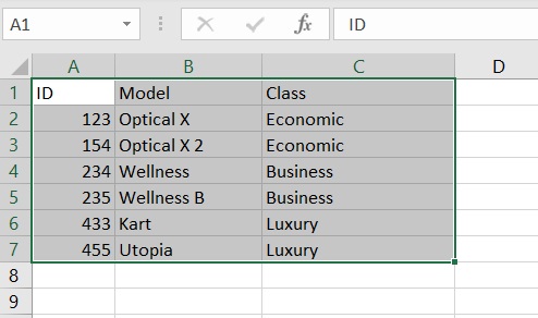
The excel sheet from which we want to import the data opens. We select the table to import and copy it (CTRL + C).

Now let’s open a session on R and enter the following command:
> tab <- read.table("clipboard", header=T, sep="\t")
> tab
   ID       Model    Class
1 123   Optical X Economic
2 154 Optical X 2 Economic
3 234   Wellness  Business
4 235  Wellness B Business
5 433        Kart   Luxury
6 455      Utopia   Luxury
Now the table data is in the form of a very common dataframe.
As you can see, the read.table() function allows us to read the data present in the temporary memory, the clipboard. If the table has headers to import, as in our case, it sets TRUE to the header key passed as a parameter. Furthermore, being an Excel sheet, the separator character “\ t” which corresponds to the TAB is selected.
To get the names of the headers we use the names() function.
> names(tab)
[1] "ID"    "Model" "Class"
Reading CSV files
Another type of file that contains tabular data is that contained in CSV files. Again you can use the read.table() function.
> models <- read.table(file="models.csv", header=T, sep=";")
> models
   ID       Model    Class
1 123   Optical X Economic
2 154 Optical X 2 Economic
3 234   Wellness  Business
4 235  Wellness B Business
5 433        Kart   Luxury
6 455      Utopia   Luxury
Import data directly from the web
But today, most of the data is on the web. There are some sites, which we could define as data sources, that every data scientist should know as sources of useful data.
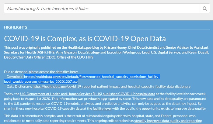
One of these is data.gov, a site that provides a lot of public data from the US. For example, on the page recently loaded, data on Covid 19 are available.

For example we select the link of the CSV containing the data on covid 19. Make a copy of it and then pass it as a parameter of the read.csv() function.
> covid19 <- read.csv("https://healthdata.gov/sites/default/files/reported_hos$The system will take some time to download all the data from the link and convert it to a dataframe. Once you get the > prompt again, the platform will be ready to accept commands again. The loaded table is a huge amount of data. For example if we want to know the size of the dataframe, we use the dim() function.
> dim(covid19)
[1] 87369    93
As we can see, the loaded dataframe has over 80,000 rows and 93 columns. Once we know the dataframe and understand which columns and rows are we are interested in, we can extract a new dataframe from the total one that contains only the data that interest us.
df <- covid19[1:100,c(1:10,68)]This is just one of the many possibilities to make a selection. In this case we select the first 100 rows (1: 100) and leave only the first 10 columns with the addition of the 68 column.
Export the data frames as CSV
With R it is also possible to perform the reverse operation. That is, once the data has been processed in a dataframe within the R platform, it can be exported as a CSV file.
write.table(models, "models2.csv")A new CSV file containing the tabular data of the dataframe will be generated in the workspace directory.
