Regularization is a technique used in regression analysis to prevent overfitting and improve the generalization ability of the model. Overfitting occurs when the model overfits the training data, also capturing the noise in the data rather than just the underlying patterns. This can lead to a poor generalization ability of the model on new data.
Ridge and Lasso regularizations
Let’s consider a standard linear regression, (OLS – Ordinary Least Squares), which is based on the following assumptions:
- Minimizes the sum of squared errors (SQE) between predicted values and observed values.
- It does not apply any penalties to the coefficients.
There are two basic Advanced Regression techniques that are based on regularization:
- Ridge regularization (L2 regularization)
- Lasso regularization (L1 regularization)
Ridge Regression and Lasso Regression techniques are variations of standard linear regression with the addition of regularization terms to limit the complexity of the model to the objective function of the regression, which affects the coefficients of the variables.
Ridge Regularization (L2 Regularization)
In Ridge regularization, a penalty term proportional to the square of the absolute values of the model coefficients (objective function) is added. The goal is to keep the coefficients small but non-zero. This helps prevent overfitting and makes the model more stable. The objective function with Ridge regularization is given by:


where 


Lasso Regularization (L1 Regularization):
In Lasso regularization, a penalty term proportional to the absolute value of the model coefficients (objective function) is added. Unlike Ridge regularization, Lasso regularization can cause some coefficients to become exactly zero, making the model more interpretable and automatically selecting a subset of the variables. The objective function with Lasso regularization is given by:


where [late] \lambda [/latex] is the regularization parameter and
The choice of the regularization parameter ( \lambda ) is crucial. Higher values of
In practice, the main difference between Ridge and Lasso is the type of rule used to penalize the coefficients. Ridge uses the L2 norm, which penalizes large coefficients without canceling them. On the other hand, Lasso uses the L1 norm, which has the property of canceling out some coefficients making them exactly zero. Thus, Lasso can be used for feature selection, while Ridge tends to keep all coefficients, even if it reduces them.
In your case, the synthetic dataset may not clearly highlight the differences between the three models, since it was generated with a quadratic term. In real-world situations with more complex data, Ridge and Lasso may prove to be useful in managing multicollinearity and selecting the most important features.
An example of regularization in Python
In this example, we are generating synthetic data with a quadratic term to demonstrate the effectiveness of polynomial regression. Next, we split the data into a training set and a test set.
The code includes standard linear regression and two types of regularization: Lasso (L1) and Ridge (L2). Let’s look at how the model coefficients are affected by regularization.
Finally, the plot_coefficients function displays the model coefficients after training. You will notice that some coefficients become exactly zero with Lasso, demonstrating the ability to automatically select the most relevant features
import numpy as np
import matplotlib.pyplot as plt
from sklearn.linear_model import LinearRegression, Lasso, Ridge
from sklearn.model_selection import train_test_split
from sklearn.preprocessing import PolynomialFeatures
from sklearn.pipeline import make_pipeline

# Let's create synthetic data
np.random.seed(42)
X = 2 * np.random.rand(100, 1)
y = 4 + 3 * X + 1.5 * X**2 + np.random.randn(100, 1)

# We divide the data into training sets and test sets
X_train, X_test, y_train, y_test = train_test_split(X, y, test_size=0.2, random_state=42)

# Function to train and visualize the model
def train_and_plot(model, X, y, title):
    model.fit(X, y)
    y_pred = model.predict(X)

    plt.scatter(X, y, color='blue', label='Actual data')
    plt.plot(X, y_pred, color='red', label='Model prediction')
    plt.title(title)
    plt.legend()
    plt.show()

# Function to display model coefficients in numerical form
def print_coefficients(model, title):
    coefficients = model.coef_.ravel()
    print(f"{title} Coefficients:")
    for i, coef in enumerate(coefficients):
        print(f"Coefficient {i + 1}: {coef}")
    print()

# Standard linear regression
linear_model = LinearRegression()
train_and_plot(linear_model, X_train, y_train, 'Linear Regression')
print_coefficients(linear_model, 'Linear')

# Regression with L1 regularization (Lasso)
lasso_model = Lasso(alpha=0.1)
train_and_plot(lasso_model, X_train, y_train, 'Lasso Regression')
print_coefficients(lasso_model, 'Lasso')

# Regression with L2 regularization (Ridge)
ridge_model = Ridge(alpha=1.0)
train_and_plot(ridge_model, X_train, y_train, 'Ridge Regression')
print_coefficients(ridge_model, 'Ridge')
Running the code gives you the three different graphs.
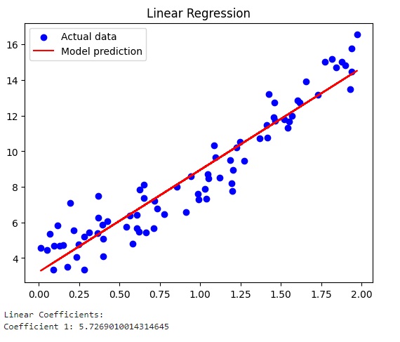
The graph relating to Linear Regression with the coefficient value equal to 5.72
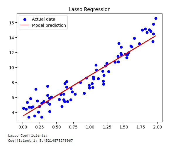
The graph relating to the Lasso regularization.
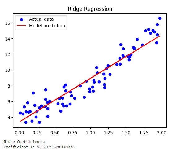
And finally the graph relating to Ridge regularization