OpenCV & Python - Edge Detection and Image Gradient Analysis

Post Views: 37,575

Introduction

In this article, the analysis of the edges and gradients of an image will be discussed. You will see how to apply some filters to an image in order to obtain a new image where the edges and the gradients are well shown. These filters, based on Laplacian derivative, will be useful tools for your image analysis, and a perfect starting point for the edge detection.

The theory of gradients images

Among the various operations that can be applied to the images, there are the convolutions of an image in which certain filters are applied to edit the image in order to obtain information or some other utility. You have already seen that an image is represented as a large numerical matrix in which the colors of each pixel of the image are represented by a number from 0 to 255 within the matrix. The convolutions process all these numerical values, by applying a mathematical operation (image filter) to produce new values in a new matrix of the same size.

One of these operations is precisely the derivative. In simple words the derivative is a mathematical operation that allows you to get the numerical values indicating the speed at which a value changes (in space, time, etc ..).

How could the derivative be important in the case of the images? You are interested in color variation called gradient.

Being able to calculate the gradient of a color is an excellent tool to calculate the edges of an image. In fact, your eye is able to distinguish the outlines of a figure present in an image thanks to the jumps between one color to another. In addition, your eye is able to perceive the depths thanks to the various shades of color ranging from light to dark, which is precisely the gradient.

From all this it is quite clear how much can be important to measure the gradient present in an image and also detect the edges of the figures with a simple operation (filter) carried out on an image.

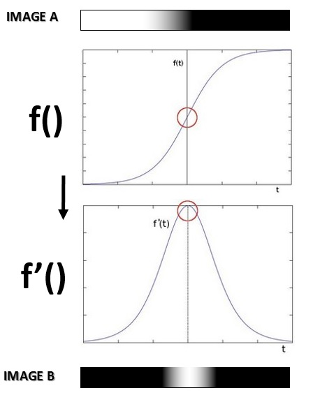
To get a better look at it from a mathematical point of view, look at this example.

As you can see from the figure, an edge is no more than a quick transition from one hue to another of a color. To simplify, the 0 is black and 1 is white. All shades of gray will be between 0 and 1.

If you put all corresponding to the gradient values in a chart ottenai the function f (). As you can see in correspondence of the edge there is a sudden transition from 0 to 1.

The derivative of the function f () and get the function f ‘(). As you can see, where you have the maximum variation of hue will have values close to 1. So converting in color, you’ll get a figure in which the white color will indicate the edge of the figure.

The calculation of the derivative – The derivative of Shobal and the Laplacian

If you are interested in how you can calculate the derivative of a matrix you can read this section, otherwise you can go directly to the case study below.

The derivative of a matrix is calculated by an operator called the Laplacian, in honor of Laplace, a famous mathematician.

$\Delta src = \frac{\partial ^2{src}}{\partial x^2} + \frac{\partial ^2{src}}{\partial y^2}$

Unfortunately the partial derivatives can not be solved analytically but must be treated with the numerical calculation using approximations. So if you want to calculate a Laplacian, you will need to calculate first two derivatives, called derivatives of Sobal, each of which takes into account the gradient variations in a certain direction: one horizontal, the other vertical.

horizontal derivative of Sobal (Sobal x). Is obtained through the convolution * The image with a matrix $G_ {x}$ kernel call always odd sizes. The simplest case, the one with the size 3 kernel is the following case:

Horizontal Sobal derivative (Sobal x). It is obtained through the convolution * of the image I with a matrix $G_{x}$ called kernel which has always odd size. The kernel with size 3 is the simplest case:

$G_{x} = \begin{bmatrix} -1 & 0 & +1 \\ -2 & 0 & +2 \\ -1 & 0 & +1 \end{bmatrix} * I$

Vertical Sobal derivative (Sobal y). It is obtained through the convolution * of the image I with a matrix $latex G_{y} $ called kernel which has always odd size. The kernel with size 3 is the simplest case:

$G_{y} = \begin{bmatrix} -1 & -2 & -1 \\ 0 & 0 & 0 \\ +1 & +2 & +1 \end{bmatrix} * I$

So in the end to get the Laplacian (approximation) you will need to combine the two previous results

$G = \sqrt{ G_{x}^{2} + G_{y}^{2} }$

although sometimes you’d prefer to also simplify this equation:

$G = |G_{x}| + |G_{y}|$

The lower the size of the kernel, the greater the approximation with which you’ll get the results. But at the same time the larger the size of the kernel the greater the required calculation. For a kernel size 3, however, the approximation can be really excessive, and it is better to use the Scharr function (also available in OpenCV). As for the examples in this article, you will use a size 5 kernel that is a good compromise calculation-approximation.

The Scharr function has these two kernels:

$G_{x} = \begin{bmatrix} -3 & 0 & +3 \\ -10 & 0 & +10 \\ -3 & 0 & +3 \end{bmatrix} G_{y} = \begin{bmatrix} -3 & -10 & -3 \\ 0 & 0 & 0 \\ +3 & +10 & +3 \end{bmatrix}$

Before you start

First to run the code in this article, certain requirements must be met.

Activate the virtual environment in which you have compiled and installed the OpenCV library.

source ~/.profile
workon cv
(cv) $

If you have not yet installed OpenCV, follow the installation procedure described in this article.

In addition, to improve the display of multiple images at once, you will use the matplotlib library. If you have not yet installed on your virtual environment, you can do this by typing

pip --no-cache-dir install matplotlib

Then install the Tkinter package required for the proper functioning of matplotlib.

sudo apt-get install python-tk

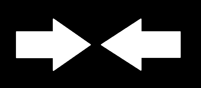
Finally, download the test image that will serve you well to see the effect of edge detection in a black and white system. Save it as blackandwhite.jpg.

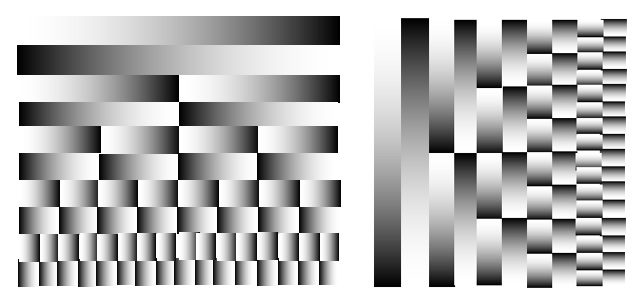
Then you’ll use an image containing gradients, download it and save it as gradient.jpg.

Also at the end you do some testing even on a color image, full of edges and color gradients. Download the following file (if you have not already done in the previous examples), and save it as logos.jpg.

Edge detection

Type the following code for the practical case.

import cv2
import numpy as np
from matplotlib import pyplot as plt

img = cv2.imread('blackandwhite.jpg',0)

laplacian = cv2.Laplacian(img, cv2.CV_64F)
sobelx = cv2.Sobel(img,cv2.CV_64F,1,0,ksize=5)
sobely = cv2.Sobel(img,cv2.CV_64F,0,1,ksize=5)

plt.subplot(2,2,1),plt.imshow(img,cmap = 'gray')
plt.title('Original'), plt.xticks([]), plt.yticks([])
plt.subplot(2,2,2),plt.imshow(laplacian,cmap = 'gray')
plt.title('Laplacian'), plt.xticks([]), plt.yticks([])
plt.subplot(2,2,3),plt.imshow(sobelx,cmap = 'gray')
plt.title('Sobel X'), plt.xticks([]), plt.yticks([])
plt.subplot(2,2,4),plt.imshow(sobely,cmap = 'gray')
plt.title('Sobel Y'), plt.xticks([]), plt.yticks([])

plt.show()

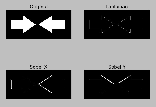
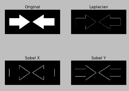
By running the code you get the following picture with 4 boxes in which the first is the original image in black and white, while the other three are the result of the three filters applied to the image.

As regards the Sobel filters, edge detection is perfect, even if limited horizontally or vertically. The diagonal lines are visible in both cases since they have both horizontal and vertical components, but the horizontal edges in the Sobel X and those in the vertical Sobel Y are not detected in any way.

Combining the two filters (the calculation of two derivatives) to obtain the Laplacian filter, the determination of the edges is omnidirectional but has some loss of resolution. In fact you can see the ripples corresponding to the edges are more subdued.

The coloring in gray is very useful for detecting both edges that the gradients, but if we are interested in only detect edges, dovari set as output an image file in cv2.CV_8U.

So you can change the type of output data from cv2.CV_64F to cv2.CV_8U in the filters function of the previous code,

laplacian = cv2.Laplacian(img, cv2.CV_8U)
sobelx = cv2.Sobel(img,cv2.CV_8U,1,0,ksize=5)
sobely = cv2.Sobel(img,cv2.CV_8U,0,1,ksize=5)

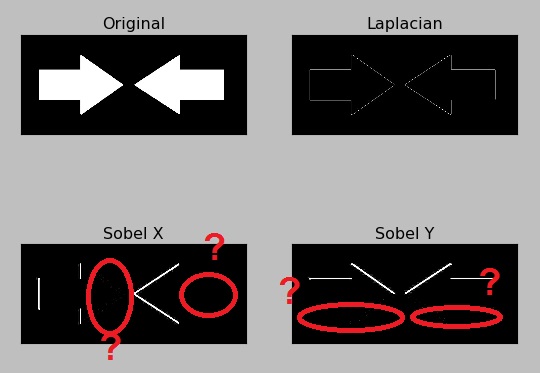
By running the code you’ll get the results in black and white, where the edges of the figures are displayed in white on a black background.

But if you look carefully at the panels of the Sobel filter X and Y you will notice right away that something went wrong. Where have some edges gone?

In fact, there was a problem while converting data. The gradients reported in the gray scale with cv2.CV_64F values are represented by positive values (positive slope) when changing from black to white. While they are represented by negative values (negative slope) when switching from white to black. In the conversion from cv2.CV_64F to cv2.CV_8U, all negative slopes are reduced to 0, and then the information relating to those edges are lost. When the program will display the image, the edges from white to black will not be represented.

To overcome this, you should keep the data in the output of the filter in cv2.CV_64F (instead cv2.CV_8U), then calculate the absolute value, and finally do the conversion in cv2.CV_8U.

laplacian64 = cv2.Laplacian(img, cv2.CV_64F)
sobelx64 = cv2.Sobel(img,cv2.CV_64F,1,0,ksize=5)
sobely64 = cv2.Sobel(img,cv2.CV_64F,0,1,ksize=5)

laplacian = np.uint8(np.absolute(laplacian64))
sobelx = np.uint8(np.absolute(sobelx64))
sobely = np.uint8(np.absolute(sobely64))

And now, if you execute the code you’ll get the right representation in white on the black edges of the figures.

Now the edges which do not appear in Sobel Sobel X and Y because parallel to the direction of detection (horizontal and vertical) are noticed well

Let’s look at gradients

In addition to the edges, you see that the Laplacian and Sobel filters are also able to detect the level of gradients across a gray scale. Apply what you’ve seen with the gradient.jpg image.

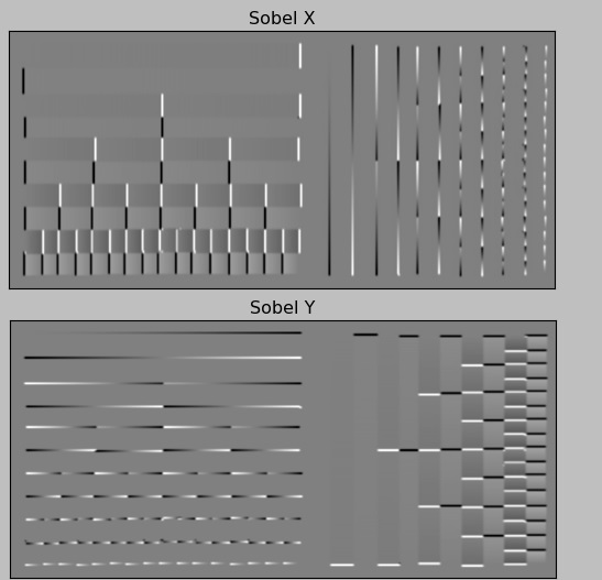
In the figure, you can see as well as the absence of gradient is represented by an intermediate gray. While the increase of the speed gradient in the transition from white to black, the figure uses a gray getting darker as indicator. While the reverse, for the transition from black to white, the figure uses an increasingly gray. Until you get in both cases at the edges (jumping from white to black, and vice versa) marked with black and white respectively.

Now, try even on a real image rich in color code and edges such as logos.jpg, and you’ll get the following figure:

OpenCV-filtri-per-la-ricerca-del-gradiente-di-immagini

Conclusion

In this article you’ve seen how the OpenCV library offers you a range of tools for the analysis of the gradients and the edge detection, ie a series of filters to apply to the images. In other articles of OpenCV series you will know more about or see other very interesting cases to analyze the images.[:]

OpenCV & Python – Edge Detection and Image Gradient Analysis